[The Principles of Diffusion Models] ( Part A )

📑 [The Principles of Diffusion Models] 시리즈

• 1️⃣ ( Part A ) 이해하기
• 2️⃣ ( Part B ) CH 2. VAE
• 3️⃣ ( Part B ) CH 2. DDPM (with VAE)

 

 

 

 

 

시작하기에 앞서 ..

 

최근 일하면서 , 논문 작성하고 , 교육듣고.... (서버를 날려먹는 사고를..) 하다보니까 정신이 하나도 없어서 공부 자체를 깊게 못했는데 틈틈히 시간을 빌려서 The Principles of Diffusion Models 라는 최신 논문을 쭉 잡고 읽어볼까 한다. 또, 기록을 남겨서 많은 사람들이 참고했으면 좋겠다는 생각으로 정리하고자 한다. 디퓨전 뿐만 아니라 생성형 모델에 깊게 빠져보는 시간을 가지고 , 인사이트를 얻고자 한다. ( 슬슬 디퓨전에 대해서 기억이 가물가물하다.. )

 

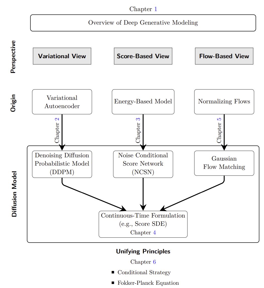
일단 위 논문은 디퓨전에 유명한 저자들이 수학적 원리와 발전과정을 매우 체계적으로 정리한 논문이다. VAE , EBM , Nomrlaizing Flow 에서 출발해 variational, score-based, flow-based 관점으로 연결시키며 설명한다. 또 , 디퓨전의 샘플링 속도나 직접 학습하고 구현하는 방법을 구조적으로 정리하고 있다.

( 최근에 직접 디퓨전을 구현하는 해외 스터디를 참가한 적이 있는데 글 작성하면서 추가적으로 정리하도록 하겠다. ) 

 

읽다가 이해가 안가거나 오타가 있거나 , 논리적으로 틀린 부분이 있으면 말씀해주세요

 

먼저 논문에서는 크게 3가지를 통해서 diffusion model 을 이해하고 심층적으로 이해할 수 있도록 돕는다고 명시되어 있다. 

• Varitational View
• Score-Based View
• Flow-Based View 

이 3개를 각각 배운 뒤 ch6 에서 위 3가지 파트가 깊게 연관되어 있음을 배울 수 있다. 

 

로드맵

cf.  기호가 이해가 가지 않는다면 Notations 을 참고하면 좋다. ( 논문들마다 기호에 대한 의미가 조금씩 다르거나 자기 스타일대로 쓰는 경우가 있어서 헷갈린다면 참고하는게 좋다. ) 

 

다 설명하기 보다 최대한 핵심 내용 위주로 정리하고자한다 ( 양이 좀 많다. ) 

 

 

Part A : Introduction to Deep Generative Modeling 

 

Deep Generative Models ( DGM ) 

- 입력 : high-dimension data ( 이미지 , 텍스트 , 오디오 등.. ) 

- 역할 : 해당 데이터들이 따르는 확률 분포 전체를 학습한다. 

- 확률 분포 ( probaility distribution )  : 데이터가 생성되는 규칙 

ex ) 

P_data : 진짜 세상의 분포 ( 이세상에 존재하는 모든 고양이 이미지의 규칙 ) -> 우린 이걸 알 수 없음 

P_phi (모델분포) : 모델이 생성한 분포 ( 여기서 phi = 모델의 모든 학습가능한 파라미터 ) 

 

1. P_data 를 알 수 없으니 ( 현실적으로 불가능하니 ) 

2. 유한개의 데이터샘플(P_data_hat) 을 가지고 P_data 를 추정하겠다 어떻게 ? 

3. loss function 을 통해서 P_phi 를 찾는다. 

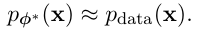
이렇게 하면 P_phi 가 P_data 를 근사할 수 있다 . 

 

(  P_phi(x) , P_Data(x) 는 모두 확률"분포".  ) 

 

그래서 이 모델 (DGM) 은 단순히 분류같은 걸 하는게 아니라 

- 출력/능력 : 그 분포에서 새로운 샘플 x 를 뽑을 수 있게 해주는 모델이다. 

데이터에서 숨겨진 분포를 학습한뒤 분포를 근사해서 새 데이터도 만들어 낼 수 있는 것이다 !

 

( 이걸 얼마나 잘 하느냐에 따라서 생성모델의 능력이 달라진다. 

데이터가 유한하기 떄문에 데이터는 discrete 할수밖에 없는데 학습을 통해서 이 데이터의 분포를 학습하면 학습된 모델은 discrete 하지 않은 데이터에 대해서도 생성하는 능력이 생긴다고 이해하면 편할듯? ) 

+ 추가로 데이터셋은 진짜 분포 P_data(x) 에서 독립 으로 나온것이라고 가정 ( i.i.d sample ) 

 

 

1.1 what is Deep Generative Modeling ? 

DGM 의 목표 

1. Realistic Generation : 진짜 데이터 처럼 보이는 샘플 생성

2. Controllable Generation :  랜덤하게 뽑는게 아니라 원하는 방향으로 제어할 수 있도록 하는것.

 

 

1.1.1 mathematical Setup 

왼쪽 ( 실제 데이터 분포 ) 를 우리가 잘 만들고 싶은것이 목표.

Goal of DGM. 

위에서도 이야기 했듯이 P_t(X) 로 P_data(x) 를 근사하는것이 목적이다. 이때 tractable 할 수있어야한다 ( 수학적 ( 계산적으로 ) 다룰 수 있어야함 - P_theta(x) 를 계산한다던가 , 샘플링 한다던지 )  . 

 

Capability of DGM.

P_theta(x) 가 있으면 할 수 있는 것들 

1. 샘플링 

2. Likelihood 평가 

 

Training of DGM 

둘간의 차이의 최소를 가지는 파라미터를 찾자 ( argmin )

DGM 의 학습방법은 모델 파라미터를 진짜분포(P_data) 와 가짜모델 (P_theta ) 사이의 차이를 줄이는 것이다. 

따라서 둘의 최소가 되도록 파라미터를 학습시키는 것이다. 

 

 

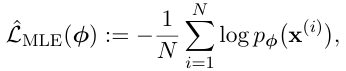
Forward KL and Maximum Likelihood Estimation (MLE).

가장 기본이 되는 수식들을 소개하고 간다. 

KL divergence ( forward KL )

가장 기본이 되는 KL divergence 의 수식이다. 

중요 포인트 : 비대칭이다.

 

< minimizing D_kl(pdata∥pϕ) encourages mode covering > 

그냥 이해하기는 어려울 수 있어서 적당히 해설을 달아볼까한다. 

 

만약에 데이터 분포에서 P_data(A) > 0 인 어떤 집합 A 가 있는데 , 모델 분포가 그 영역에서 P_t(x) = 0 이라면 수식상 
log(P_data(A) / 0 ) -> +inf 로 발산하게 되고 KL 이 무한대가 된다.

 

이게 쉽게 설명해서 무슨말이냐고 하면

- 어떤 영역 A 에서 데이터가 아주 가끔 나오는데 ( P_data(A) > 0 ) 

- 모델이 여기서는 데이터가 안나온다고 하면 ( P_t(x) = 0 ) 으로 설정되고 ( 이럼 로그가 발산해버림 ) 

- 그 영역에서 KL 이 무한대가 되어버린다. 

 

이렇게 되면 KL 을 최소화해야하는 입장에서  "데이터가 실제로 나오는곳 P_data(x) > 0 에 절대 확률 0을 두면 안되게 한다. "

( 왜? 너무 커지니까 ! ) 

 

이런 행동을 mode covering 이라고 부른다.

mode 란 봉우리를 말하는데 forward KL 은 모든 봉우리를 유지하려고 노력한다 ( 없으면 너무 큰 패널티가 있기 때문 ) 

 

다시 돌아가서. 그래서 이러한 이유로 D_KL(p_data || p_t ) 를 사용하게 되는것이다. 

 

cf.  kl divergence & moe covering 에 대해서는 추가적으로 블로그 참조. 

https://angeloyeo.github.io/2020/10/27/KL_divergence.html 

https://process-mining.tistory.com/147

 

 

 

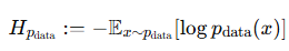
다시 KL 로 돌아와서 아까는 보지 못했던 H(p_data) 가 생겼는데 이는 데이터 분포의 엔트로피라서 파라미터와 상관없는 상수이다. 따라서 우리가 조절할 수 있는 부분은  log(P_t(x)) 의 기대값이다. 

 

그렇다면 수식을 이렇게 바꿀 수 있는데 

 

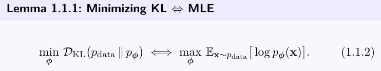
Forward KL 을 최소화 하는것 <=> 데이터에 대한 평균 log-likelihood 를 최대화 하는 것과 같다. 

(Kl min <-> MLE) 

 

cf. 

forward KL  에서 결국 영향을 주는 항은 하나밖에 없다 ( E_pdata(...)) 

KL 이 모델에게  데이터가 자주 나오는  X 에서 모델도 큰 log prob 를 주라는 뜻이다. 

-> 데이터가 자주 나오는 포인트가 중요도가 높다 -> 그럼 그 x 에 대해서 모델 확률을 크게 만든다 -> logP(x) 를 크게 만든다.  ( max log p(x) ) 

 

즉, forward KL 은 데이터가 자주 나오는 곳에서 모델 확률을 크게 하도록 만들게 된다. 

결국 이런식으로 정리할 수 있게 된다. 

 

직관적인 목적으로 다시 정리하면 (with gpt )

MLE의 직관적 목적:

모델이 이 데이터를 ‘가장 잘 설명하게’ 하라.

 

Forward KL의 의미는:

모델이 데이터 분포와 같은 분포가 되도록 만들라.

둘 다 “데이터 분포를 최대한 모방”한다.

 

 

Fisher Divergence 

fisher divergence 는 score based diffusion modeling 에서 중요한 컨셉이다. 

 

--> 여기서 다 하고가면 너무 무거워서 chapter 3 를 할때 다시 정리하고자한다. (score 개념 부터해서 ... 전부다 정리 ) 

어쨌든 하나 알아야할 점은 diffusion 역시 score base 라는거 

-> ( noise 를 예측하는 방식으로 데이터분포의 score 를 학습하는 모델 ) 

 

Beyond KL

-> ch 7 에서 다시 정리

 

 

 

1.1.2 Challenges in Modeling Distributions 

다시 정리를 하자면 우리가 진짜로 하고 싶은일은 

- 진짜 데이터 분포 P_data(x) 

- 만드는 모델 P_t(x) 

목표 : P_t(x) 가 P_data(x) 를 최대한 잘 근사하도록 좋은 pdf 를 신경망으로 만든다. 그리고 이걸로 샘플링하고 likelihood 도 계산을 하자. 하지만 pdf 가 되려면 아래와 같은 두가지 조건을 만족해야한다. 

 

 

두가지 조건

 

 

step 1 : Ensuring Non-Negativity 

pϕ​(x)≥0 을 만족시키기 위해서는 네트워크 출력값 Eϕ(x) 에다가 항상 양수를 내는 함수를 씌운다. ( 절댓값 ,  제곱 , exp () ... ) 

 

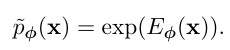
가장 흔하게 쓰는게 exponential 이라서 이렇게 나와있는듯. 그래서 이 p~​ϕ​(x) 는 항상 0보다 크다. 

하지만 아직 적분이 1 은 아니다 ( unnormalized dnesity ) 

 

 

Step 2: Enforcing Normalization.

이제 p~​ϕ​(x) 이 항상 positive 인것은 해결했지만 아직 확률밀도 (pdf) 는 아니다. 그래서 이걸 진짜 확률 밀도 함수 (pdf) 로 만들기 위해서

 

다음과 같이 스케일을 맞춰준다

분모는 다음과 같이 생기고, 

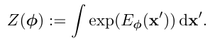
그리고 이걸 normalizing constant / partition function이라고 부른다. 

 

 

이렇게 구성하면 

분자 : 항상 양수

분모 : 전체 적분값 

 

다시 정리해보면

1. 신경망이 (Eϕ(x) ) 를 만듬.

2. exp 씌워서 p~​ϕ​(x) 만듬. 

3. 전체적분 Z(ϕ) 로 나눠서 정상적인 pdf pϕ(x) 를 만든다. 

 

간단해 보이지만 여기서 다시 문제가 생긴다. 

문제 . high-demension problem 

- 입력 차원이 너무 크다 -> 코차원 공간에 대해서 적분해야 Z(ϕ) 알 수 있다.  하지만 이 계산이 매우 어렵다. 

그래서 결국 partition function Z(ϕ) 때문에 모든 게 막히게 된다.

 

이게 모델링의 난제이다. 

 

그래서 이것을 잘 해결해 보고자 여러가지 DGM 들이 나와서 z 문제를 우회하거나 줄이는 방식으로 모델이 발전된다. 

이에 대한 더 자세한 이야기는 이야기를 진행하면서 더 설명해보도록 하겠다 .

 

 

 

 

1.2 Prominent Deep Generative Models

high-dimensional data 의 확률 분포를 잘 모델링 하고 싶은것이 생성형 모델의 큰 챌린지이다. 

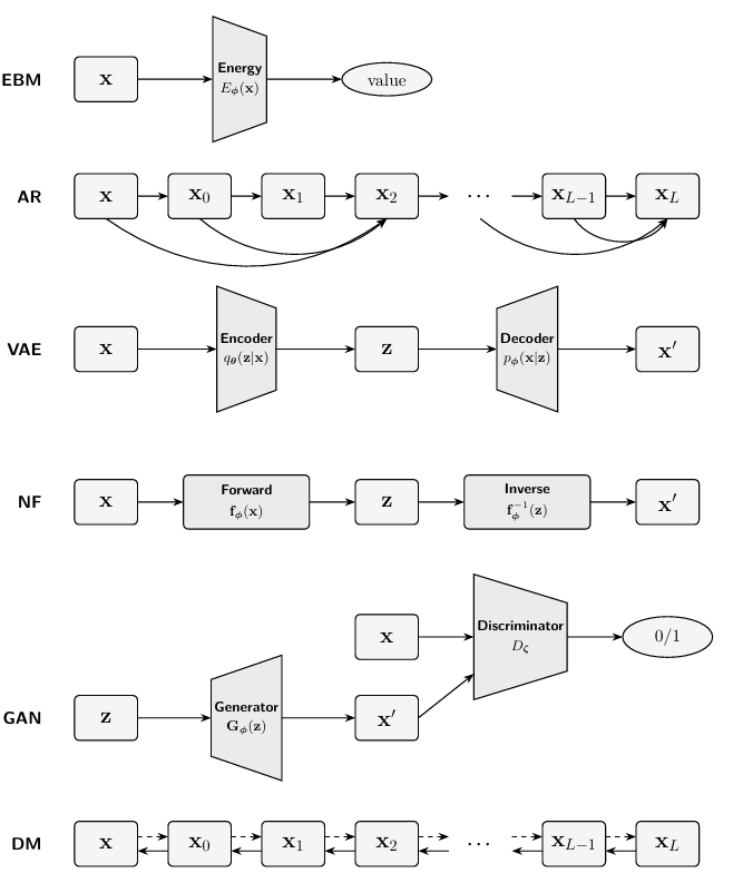
그런데 normalization , efficiency , expressiveness 에 대한 trade-off 가 각 모델마다 모두 다르다. 우의 그림 처럼 다양한 모델들이 존재한다. 여기서 다 자세하게 다루지는 않고 part B 에 가서야 각 챕터별로 깊게 들어간다. 

 

위 모델들이 매우 유명하기도 하고 기본적인 모델이기 때문에 gpt 를 돌려서 잠깐 정리만 하고 다음으로 넘어갈까한다. ( 이후에 part b 에서는 조금 더 자세히 설명해보겠다 . ) 

 

 

-> 궁금하다면 해당 부분을 그대로 붙여넣기해서 gpt 에게 설명해달라고 하자. 

 

[role] 아래 본문을 자세하게 설명할 것. 그리고 아래 명시한 내용은 반드시 설명할것.

(반드시 설명시 포함시켜야 될 부분 )
1. EBMs -> diffusion 과 연결되는 부분 
2. VAE 에서 elbo 에 대한 간단한 설명 

3. “flow-based 개념(연속적인 변환, ODE/SDE)을 빌리되,
invertible 제약이나 Jacobian 계산 부담은 줄이고,
확률분포는 score 기반으로 다루는 방식”  --> 이 부분에 대해서 

[본문]
Energy-Based Models (EBMs). EBMs (Ackley et al., 1985; LeCun et al.,
 2006) define a probability distribution through an energy function Eϕ(x) that
 assigns lower energy to more probable data points. The probability of a data
 point is defined as:
 pϕ(x) := 1
 Z(ϕ) exp(−Eϕ(x)),
 where
 Z(ϕ) = exp(−Eϕ(x))dx
 is the partition function. Training EBMs typically involves maximizing the
 log-likelihood of the data. However, this requires techniques to address the
 computational challenges arising from the intractability of the partition func
tion. In the following chapter, we will explore how Diffusion Models offer an
 alternative by generating data from the gradient of the log density, which does
 not depend on the normalizing constant, thereby circumventing the need for
 partition function computation.
 Autoregressive Models. Deep autoregressive (AR) models (Frey et al., 1995;
 Larochelle and Murray, 2011; Uria et al., 2016) factorize the joint data
 distribution pdata into a product of conditional probabilities using the chain
 rule of probability:
 D
 pdata(x) =
 i=1
 pϕ(xi|x<i),
 where x = (x1,...,xD) and x<i = (x1,...,xi−1).
 Each conditional pϕ(xi|x<i) is parameterized by a neural network, such as a
 Transformer, allowing flexible modeling of complex dependencies. Because each
 term is normalized by design (e.g., via softmax for discrete or parameterized
 Gaussian for continuous variables), global normalization is trivial.
1.2. Prominent Deep Generative Models
 23
 Training proceeds by maximizing the exact likelihood, or equivalently
 minimizing the negative log-likelihood,
 While AR models achieve strong density estimation and exact likelihoods,
 their sequential nature limits sampling speed and may restrict flexibility due
 to fixed ordering. Nevertheless, they remain a foundational class of likelihood
based generative models and key approaches in modern research.
 Variational Autoencoders (VAEs). VAEs (Kingma and Welling, 2013) ex
tend classical autoencoders by introducing latent variables z that capture
 hidden structure in the data x. Instead of directly learning a mapping between
 x and z, VAEs adopt a probabilistic view: they learn both an encoder, qθ(z|x),
 which approximates the unknown distribution of latent variables given the
 data, and a decoder, pϕ(x|z), which reconstructs data from these latent vari
ables. To make training feasible, VAEs maximize a tractable surrogate to the
 true log-likelihood, called the Evidence Lower Bound (ELBO):
 LELBO(θ,ϕ;x) = Eqθ(z|x) [logpϕ(x|z)] − DKL (qθ(z|x)∥pprior(z)).
 Here, the first term encourages accurate reconstruction of the data, while the
 second regularizes the latent variables by keeping them close to a simple prior
 distribution pprior(z) (often Gaussian).
 VAEs provide a principled way to combine neural networks with latent
variable models and remain one of the most widely used likelihood-based
 approaches. However, they also face practical challenges, such as limited
 sample sharpness and training pathologies (e.g., the tendency of the encoder
 to ignore latent variables). Despite these limitations, VAEs laid important
 foundations for later advances, including diffusion models.
 Normalizing Flows. Classic flow-based models, such as Normalizing Flows
 (NFs) (Rezende and Mohamed, 2015) and Neural Ordinary Differential Equa
tions (NODEs) (Chen et al., 2018), aim to learn a bijective mapping fϕ
 between a simple latent distribution z and a complex data distribution x via
 an invertible operator. This is achieved either through a sequence of bijective
 transformations (in NFs) or by modeling the transformation as an Ordinary Dif
ferential Equation (in NODEs). These models leverage the “change-of-variable
 formula for densities”, enabling MLE training:
 log pϕ(x) = logp(z) +logdet ∂f−1
 ϕ (x)
 ∂x ,
24
 Deep Generative Modeling
 where fϕ represents the invertible transformation mapping z to x. NFs explicitly
 model normalized densities using invertible transformations with tractable
 Jacobian determinants. The normalization constant is absorbed analytically
 via the change-of-variables formula, making likelihood computation exact and
 tractable.
 Despite their conceptual elegance, classic flow-based models often face prac
tical limitations. For instance, NFs typically impose restrictive architectural
 constraints to ensure bijectivity, while NODEs may encounter training ineffi
ciencies due to the computational overhead of solving ODEs. Both approaches
 face challenges when scaling to high-dimensional data. In later chapters, we
 will explore how Diffusion Models relate to and build upon these classic
 f
 low-based methods.
 Generative Adversarial Networks (GANs). GANs (Goodfellow et al., 2014)
 consist of two neural networks, a generator Gϕ and a discriminator Dζ, that
 compete against each other. The generator aims to create realistic samples
 Gϕ(z) from random noise z ∼ pprior, while the discriminator attempts to
 distinguish between real samples x and generated samples Gϕ(z). The objective
 function for GANs can be formulated as:
 min
 Gϕ 
max
 Dζ 
Ex∼pdata(x)[logDζ(x)]
 real
 +Ez∼pprior(z) [log(1 − Dζ (Gϕ(z)))]
 fake
 .
 GANsdonot define an explicit density function and therefore bypass likelihood
 estimation entirely. Instead of computing a normalization constant, they focus
 on generating samples that closely mimic the data distribution.
 From a divergence perspective, the discriminator implicitly measures
 the discrepancy between the true data distribution pdata and the generator
 distribution pGϕ
 , where pGϕ 
denotes the distribution of generated samples
 Gϕ(z) obtained from noise z ∼ pprior. With an optimal discriminator for a
 f
 ixed generator Gϕ computed as
 pdata(x)
 pdata(x) + pGϕ
 (x) ,
 the generator’s minimization reduces to
 min
 Gϕ 
2DJS pdata∥pGϕ
 −log4.
 Here, DJS denotes the Jensen–Shannon divergence, defined as
 DJS(p∥q) := 1
 2DKL p p+q
 2 + 1
 2DKL q p+q
 2 .
1.2. Prominent Deep Generative Models
 25
 This shows that GANs implicitly minimize DJS(pdata ∥pGϕ
 ). More broadly,
 extensions such as f-GANs (Nowozin et al., 2016) generalize this view by
 demonstrating that adversarial training can minimize a family of f-divergences,
 placing GANs within the same divergence-minimization framework as other
 generative models.
 Although GANs are capable of generating high-quality data, their min-max
 training process is notoriously unstable, often requiring carefully designed
 architectures and engineering techniques to achieve satisfactory performance.
 However, GANs have since been revived as an auxiliary component to enhance
 other generative models, particularly Diffusion Models 

 

 

 

1.3 Taxonomy of Modelings

DGM 을 어떻게 확률 분포를 정의하는가 ? 를 기준으로 두 그룹으로 나눈다. 

 

DGM 은 결국 둘중 하나이다. 

1. Explicit model

2. Implicit model 

-> 둘의 차이는 P(x) 를 명시적으로 정의하냐 아니면 msapling 을 통해서 하나만 정의하냐의 차이이다. 조금 더 자세히 알아보자.

 

 

1) Explicit models 

정의 : 모델이 직접 pϕ(x) 를 정의한다. ( p(x) 가 수식으로 존재 ! )

예시 : AR , NF , VAE , Diffusion model 

 

1. 정확한 확률 밀도를 계산할 수 있거나 

2. 확률에 대한 tractable bound 를 계산  ( diffusion 에서 학습은 ELBO / 추론에서 p(x) 는 어려워도 bound 존재 ) 

3. 확률에 대한 approximation 을 계산.  ( VAE 에서 ELBO ) 

 

 

2) Implicit model 

정의 : 직접 정의 하지 않고 "샘플 생성 과정"만 정의한다. 

예시 : GAN 

 

GAN 같은 경우는 확률밀도가 존재하지 않고 / 미분(계산) 이 불가능하다 ( intractable ) 

그래서 이 모델은 확률을 정의하지 않고 그냥 샘플을 만들어 내는 함수만 정의한다. 

-> 그래서 gan 을 구현하는게 꽤나 어려운 일이였을지도. 

-> 샘플은 주지만 likelihood 는 없음 . 

 

 

그래서 디퓨전은 어디에 있는가 ? 

- 앞에서도 이야기 했지만 diffusion 은 explicit 모델이다. 

- 학습시에 EBLO 사용한다. 

 

논문에는 조금 더 많은 내용이 존재하기는 하나. 지금 모두 다 설명하기는 쉽지 않기 때문에 패스. 

그래도 잠깐 이야기 하자면 diffusion 은 "latent VAE + Energy base score + flow-like " 의 결합이다. 

 

(with gpt )

Diffusion이 다음 세 가지를 모두 결합했다:

1. VAE에서
   • variational training (ELBO 기반)
2. EBM에서
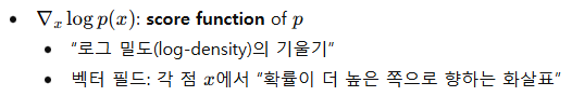
   • score = ∇ log p(x)
   • 정규화 상수(Partition function) 필요 없는 점
3. Flow에서
   • 연속-time 변환 (ODE/SDE 기반 역확산)
   • invertible mapping의 continuous analog

 

(어차피 여기서는 이해가 안가는게 정상이다. -> 하나하나씩 배우고 ch6 에서 이 내용들을 합친다고 했으니 걱정말자. ) 

이제 part a 의 내용을 마무리 짓고 하나하나씩 더 딥다이브 해보자. 

 

 

 

< Part A 의 마무리 >

 

요약

- 생성형 모델이 하고자 하는 것 : p_data 에 근사한 p_t 를 배우자 

- 그리고 거기서 문제는 정규화 상수 Z( ϕ ) 가 고차원에서 intractable 한것 

- 그래서 이걸 해결하고자 많은 방식들이 등장했다. 

- diffusion 의 핵심은 VAE + EBM + NF(normalizing flow) 이다. 

 

그래서 우리는 

1) VAE + ELBO 에 대한 개념을 배워서 DDPM 이 VAE 의 확장 형태임을 배울 것이고

2) SCORE-BASE DIFFUSION = EMB + score matching 임을 배우고 

3) diffusion 이 결국 normalizing flow 의 일반화 임을 배울것이다. 

 

나도 디퓨전을 공부하면서 디퓨전 논문을 딱 읽고 아.. 뭔가 어디서 썼던 개념이였던거 같은데 ? 이거 어디서 봤는데 ? 

라고 생각을 했었고 그런 개념들이 조금 파편화되어 있어서 명확하게 이해가 안되는 부분들이 꽤나 많았는데 이번 기회로 조금 더 명료하게 이해할 수 있는 방향을 잡은 것 같아서 매우 좋았다. 

 

또, 이 큰 흐름들을 보다보니까 이 세가지 큰 생성모델에서의 패러다임을 잘 합쳐놓은 논문인 diffusion 이 꽤나 당연하게 나온것인것 같다는 ( 말이 쉽지 ) 생각도 들고, transformer 에 대해서 교수님에게 강의를 듣다가 자기는 뭐가 특별한지 몰랐었다 당연한 흐름에서 나왔던거 같다는 말이 뭔가 와닿지 않았었는데 이런 개념을 모두 숙지한 사람에게서는 어쩌면 디퓨전이라는게 꽤나 생각의 흐름이 꽤나 자연스럽게 나왔을거라는 생각이 ( 하지만 다시봐도 대단하다 . ) 든다. 

 

part B 부터는 내용이 많아서 하나의 챕터별로 끊어서 설명할까 한다. 

그럼 다음 장에서는 VAE 에 대해서 깊게 알아보고 , VAE 는 공부한지 얼마 안되어서 필기및 유튜브에서 봤던 시각적인 자료들을 올리면서 같이 설명해보겠다.